
Table of Contents
Introduction
In every industrial process, temperature control is a necessity. Components and circuit are the most fundamental aspect that work together to achieve a desired output (Cruz & Ramírez-Figueroa 56). This lab uses LabVIEW program known as Virtual Instruments (VIs) to provide a basic method of recording reaction time to a visual stimulus. Moreover, it aims at creating Virtual Instrument (VIs) which are the LabView graphical programs made up of Front Panel and Block diagram so as to analyze and present the result for decision making (Immeran 34).Generally, the ultimate aim of the lab is to interface the thermocouple with LabVIEW to simulate a cooling system. The experiment involves the use of VIs together with thermocouple as the basic measuring element for the study. Most significantly, the choice of VIs is because its execution is data dependent hence suitable to monitor thermocouple operation within the cooling system.
As a product of National IntrumentsTM , the software system (VIs) in the experiment acquires data, controls other instruments such as thermocouple, analyzes data and finally presents the result in form of graphs. With the two major parts of the VIs, the system uses the block diagram to demonstrate the structure of the closed loop control system with the entire process aimed at establishing the reaction time ( Luciano 88).
This paper therefore organizes the report in terms of the experimental method, result, discussion and conclusion.
Experimental Method
This lab consisted of creating two VIs to complete two different functions. The first VI is able to measure the reaction time of the user by timing how long it takes a user to hit a stop button after a LED lights up green. The second VI was created to monitor a thermocouple’s readings to control a cooling system. The VI also would set off an alarm if the temperature were outside of critical boundaries. Lastly, the VI would graph the temperature as a function of time.
The first VI has a simple front panel but a complicated block diagram. The front panel is pictured below in Figure 1. The front panel takes in two inputs initially from the user. These are the names of the user and the number of trials wanted for each user to complete. The start and stop buttons control the VI. The start button starts the delay time for the LED to turn on. As soon as the LED turns on the user is supposed to hit the stop button. The data displayed on the front panel consists of the trials that have been completed, the delay time, the reaction time, which is the time it took for the user to his stop after the LED turned green, and the average reaction time.

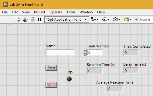
Figure 1: Reaction Time Front Panel
The front panel pictured in Figure 1 is controlled by the block diagram below in Figure 2. The first thing that happens in the code is that the trials completed, the average reaction time, the reaction time sum, the reaction time, and the delay time is all set to zero. The reaction time sum is the reaction time for each repetition that has been completed so far. Then a while loop is initiated that repeats for the number of trials specified by the user on the front panel. This is done by adding one to the number of trials completed each time a repetition is completed, which is displayed on the front panel, and comparing it to the number of trials wanted. When these numbers are equal the while loop ends and the code is stopped.
Within the while loop is a frame structure, which allows the code not to continue until each frame is completed in entirety. The first thing that happens in the frame structure is that the name of the user is taken in and the LED is turned off. The frame also has a while loop which it cannot escape until the start button is hit. As soon as the start button is hit the code progresses onto the next frame which just delays the code. The reaction time and the delay time is first set to zero while a random delay time is calculated. The code generates a random number between 0 and 1 and then multiplies that by five. Then five is added to that so that the delay time is between five and ten seconds. This time is then put into a time delay module so the code cannot continue until the delay time happens. After the code waits for the specified delay time the LED turns green, and the delay time is displayed on the front panel. The time that the LED turned on is also stored. Then, once the stop button is hit, the code is allowed to continue and the time that the stop button was hit is stored. The fourth frame turns the LED off and takes the two times that were just stored and finds the time difference between the two in seconds, which is the reaction time. This is then passed onto the next frame which first bundles both the delay time and the reaction time together, adds the name to the data, and sends it to an excel sheet to be used later. Also in this frame, reaction time sum is calculated by taking the reaction time sum from the last repetition and adding it to the reaction time. Lastly, the next frame waits for one second and calculates the average sum, which is done by dividing the reaction time sum by the number of trials that have been completed.
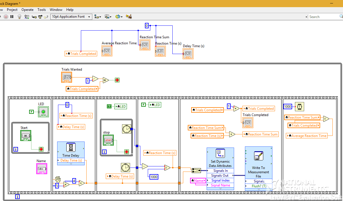
Figure 2: Reaction Time Block Diagram
Figure 3 below is the front panel for the thermocouple monitor. On the front panel, the cooling system upper and lower limit and the critical upper and lower limit can be set by the user. There are also two LEDs, which are green when the temperature is within the set bounds. The system OK LED turns blue when the temperature rises above the cooling system upper and the critical alert off LED turns red when the temperature is outside either the critical upper or lower limit. The front panel also displays a graph, which graphs the temperature versus a function of time and displays the current reading that the thermocouple is providing.
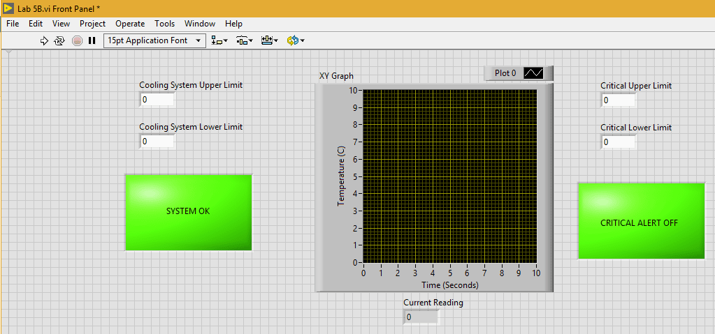
Figure 3: Thermocouple Monitor Front Panel
Lastly, the block diagram, which controls the front panel displayed in Figure 3, is displayed below in Figure 4
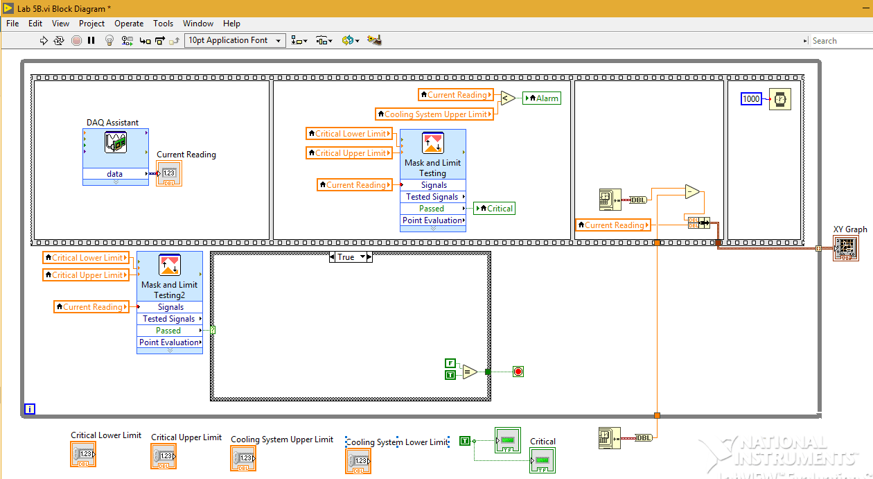
Figure 4: Thermocouple Block Diagram
Results
The VI to measure the user’s reaction time was used to measure both the reaction time and the average reaction time of each user. The VI was set to repeat 20 times for each person. This data was then graphed in a histogram for each trial with a Gaussian curve overlay. These charts were calculated by using formulas provided with in the lecture slides from week two and built in formulas within Google Sheets.
Below, in Figure 5, is the histogram from the first set of data.
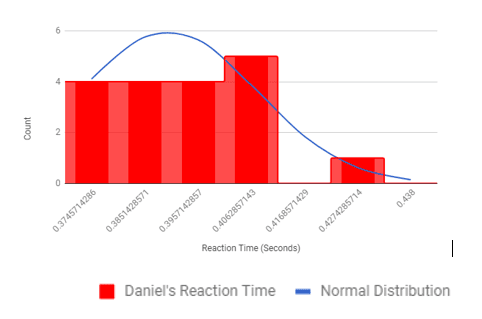
Figure 5: Trial One Reaction Time Histogram.
Figure 6, below, is the histogram from the second trial of data.
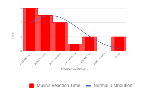
Figure 6: Trial 2 Reaction Time Histogram
The data from both reaction time tests was not only graphed as a histogram with a Gaussian curve but had a statistical analysis performed upon it. For each trial the mean reaction time, the median reaction time, the standard deviation, the error of the reading and the confidence interval was calculated. The confidence interval was calculated as a +/ – value in which the data would fall off the mean 95 percent of the time. The data from the statistical analysis is below in Table 1. All of these values were calculated using built in functions on Google Sheets except for the mean value, which was calculated by the VI.
Table 1: Reaction Time Data
| Trial Number | Mean Reaction Time | Median Reaction Time (Seconds) | Standard Deviation | Error | Confidence Interval (95%, +/- from Mean) |
| 1 | 0.371 | 0.356 | 4.37E-02 | 9.77E-03 | 2.05E-02 |
| 2 | 0.390 | 0.387 | 1.77E-02 | 3.95E-03 | 8.26E-03 |
Discussion
From the above reaction time data in table 1 , the reaction time in the second trial is higher than the first trial ( 0.390sec and 0.371 sec. respectively). Correspondingly, there is a significant reduction in deviation of confidence interval from the mean in the second trial than first. The higher the deviation of the confidence interval from the mean the higher the probability that the actual data points and the actual distribution curve fall within the 95% confidence interval hence suggests a normal distribution curve (Nasser and Kim 78). It is also noted that the measurement error on each data point are different(9.77E-03 and 3.95E-03). This suggests that the confidence bounds are not necessarily linear by nature. The larger confidence interval showed in the second trial suggest that more response time of 0.390seconds exposes the measurements to a lot of noise, thus, higher measurement error of 3.95E-03 as demonstrated in the above statistical output.
Conclusion
The operation of VIs as described in the above experiment is truly a prototype that reflects the operation of an entire cooling system or air conditioning system. Within the constraints of the experiment design, the signal error output indicates that the system actually performed within the design limits. This experiment also reveals the usefulness of using Virtual Instruments in determination of response time in such control experiment . From the different results from the two trials above, it is undoubtedly certain that the lower the response time, the better the result (Sheng and Yizhong 56). Therefore designing a temperature control system or a system of similar nature would be made easier with the help of LabVIEW application software. The experience in that regard provides a good demonstration of the actual role played by the aforementioned instrument in the design of any cooling system.
We can do it today.
- Cruz, Pedro Ponce, and Ramírez-Figueroa Fernando D. Intelligent control systems with LabVIEW. Springer, 2010.
- Catani, Luciano. “Extending LabVIEW Aptitude for Distributed Controls and Data Acquisition.” Practical Applications and Solutions Using LabVIEW™ Software, Jan. 2011, doi:10.5772/20416.
- Kehtarnavaz, Nasser, and Namjin Kim. “LabVIEW Programming Environment.” Digital Signal Processing System-Level Design Using LabVIEW, 2005, pp. 5–14., doi:10.1016/b978-075067914-5/50003-9.
- Immeran, Mohd Dzulraini. Rate of energy transfer measurement of aluminium rod using LabVIEW 8.0.
- Sheng, Ai, and Yizhong Wang. Manufacturing and engineering technology. CRC Press/Balkema, 2015.